Computing seismic kernels¶

This tutorial explains how to use persephone to compute seismic rotational kernels of evolutionary models obtained through the interface. The user will find an extensive description and discussion of the rotational kernel formalism presented in this tutorial in Chapter 8 of the book by J. Christensen-Dalsgaard, Lecture Notes on Stellar Oscillations.

import persephone as pph
import persephone.kernels.rotation as pph_rot
import pygyre
import os
pph.__version__

'0.1'

Computing the stellar model¶

In this tutorial, we will consider a \(1.3~\rm M_\odot\) stellar model along its evolution.

parameters = {"controls":{"initial_mass":"1.3",
                         "initial_z":"0.0134"}}
model_dir = "kernel_example"

The create_mesa_model function provides the wrapper necessary to run a single model in its working directory.

pph.grids.create_mesa_model (model_dir=model_dir,
                             parameters=parameters,
                             run_mesa=True, verbose=False)

Low-frequency modes computation with GYRE¶

We want to follow the evolution of the properties of low-frequencies gravity modes (g modes) of the model along stellar evolution. To do this, we need to use a dedicated GYRE input template file, as the standard input file included in persephone is dedicated to compute the properties of high-frequency acoustic modes (p modes). The customed template file to use is shown below.

Note: for the sake of consistency between filenames templates and further computation of 2D-kernels, we use GYRE to compute \(m=1\) modes, even if we do not actually include rotation in GYRE inputs (see the rot namelist below). Therefore, here, \(m=0\) and \(m=1\) mode computed by GYRE should have the exact same properties.

pph.grids.show_kernel_example_gyre_input ()

&constants
/

&model
  model_type = 'EVOL'  ! Obtain stellar structure from an evolutionary model
  file_format = 'MESA' ! File format of the evolutionary model
  add_center = .FALSE.
/

&mode
  l = 1
  m = 1
  n_pg_min = -5
  n_pg_max = 5
/

&osc
  inner_bound = 'REGULAR'
  outer_bound = 'VACUUM' ! Use a zero-pressure outer mechanical boundary condition
/

&rot
  Omega_rot_source = 'UNIFORM'
  Omega_rot = 0.
  Omega_rot_units = 'UHZ'
/

&num
  diff_scheme = 'COLLOC_GL4' ! 4th-order collocation scheme for difference equations
/

&scan
  grid_type = 'INVERSE'
  freq_min = 10
  freq_max = 300
  n_freq = 500
  freq_units = 'UHZ'
/

&grid
  w_osc = 10 ! Oscillatory region weight parameter
  w_exp = 2  ! Exponential region weight parameter
  w_ctr = 10 ! Central region weight parameter
/


&ad_output
  summary_item_list = 'l,n_pg,n_p,n_g,freq,freq_units,
                       E, E_norm, E_p, E_g, R_star, M_star,
                       Delta_p, Delta_g'
  detail_item_list = 'l,m,n_pg,n_p,n_g,omega,freq,x,xi_r,
                      xi_h,c_1,As,V_2,Gamma_1,P,rho,
                      eul_P,prop_type,
                      E, E_norm, E_p, E_g, R_star, M_star,
                      Delta_p, Delta_g, M_r'
  freq_units = 'UHZ'
  freq_frame = 'INERTIAL'
/

&nad_output
/

By default, in order to save disk memory, persephone uses a GYRE template that does not save mode details file. However, here, they are required to compute the seismic kernel, the procedure to save the detail files can be simply included in the interface by setting add_details=True. In this case, persephone will add to the input namelists above a detail_template argument and will take care of creating the directories where the detail files are stored.

_gyre_in = pph.grids.get_kernel_example_gyre_input ()
with _gyre_in as template_file :
    pph.grids.analyse_gyre (model_dir, run=True, template_file=template_file,
                            add_details=True, verbose=False)

Kernels along evolution¶

This list of details directory can then be accessed through the get_listdir_gyre_details function. Selecting a details directory, the details file can be obtained using get_detail_file.

list_details = pph.grids.get_listdir_gyre_details (model_dir, sort=True)
list_details

['kernel_example/LOGS/profile1_details',
 'kernel_example/LOGS/profile2_details',
 'kernel_example/LOGS/profile3_details',
 'kernel_example/LOGS/profile4_details',
 'kernel_example/LOGS/profile5_details',
 'kernel_example/LOGS/profile6_details',
 'kernel_example/LOGS/profile7_details',
 'kernel_example/LOGS/profile8_details',
 'kernel_example/LOGS/profile9_details']

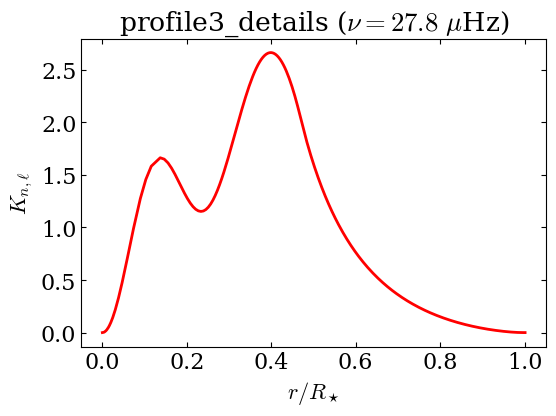
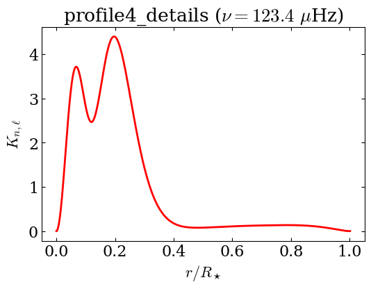
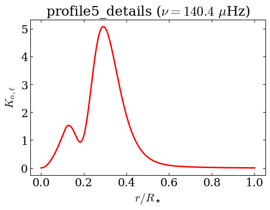
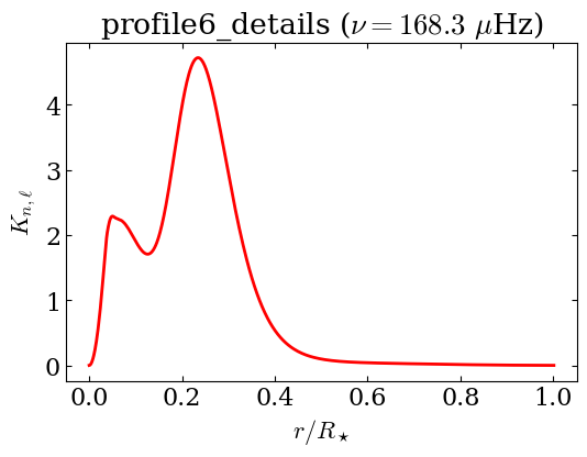
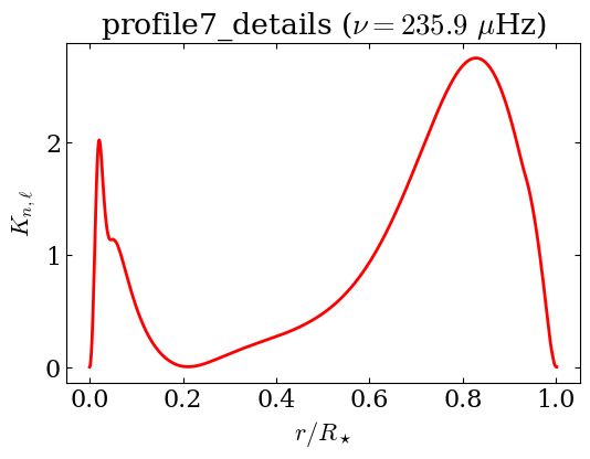
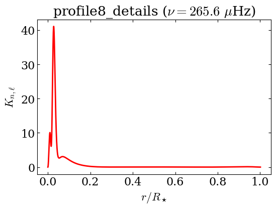
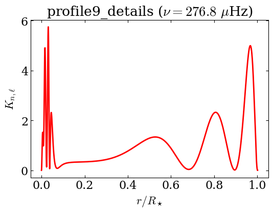
Making the approximation of shellular rotation, it is possible to compute one-dimensional kernels that do not depend on the azimuthal number \(m\). In this example, we focus on the \(n=1\) g mode of the models (if computed, see Note below).

Note: Depending on the stellar structure, not all the models we computed have the \(n=1\), \(\ell=1\) g mode in the considered frequency range, or g modes at all (if they are fully convective). For this reason, the file_exists boolean status is used to avoid FileNotFoundError exceptions.

for details_dir in list_details :
    filename, file_exists = pph.grids.get_detail_file (details_dir, n=-1, l=1, m=1)
    if file_exists :
        d = pygyre.read_output(filename)
        beta_nl, K_nl = pph_rot.compute_shellular_kernel (d["x"], d["rho"],
                                                           d["xi_r"], d["xi_h"],
                                                           l=d.meta["l"])
        title = r"{} ($\nu={:.1f}$ $\mu$Hz)".format (os.path.basename (details_dir),
                                                      d.meta["freq"].real)
        fig = pph_rot.plot_shellular_kernel (d["x"], K_nl, color="red", lw=2,
                                             title=title, figsize=(6,4))

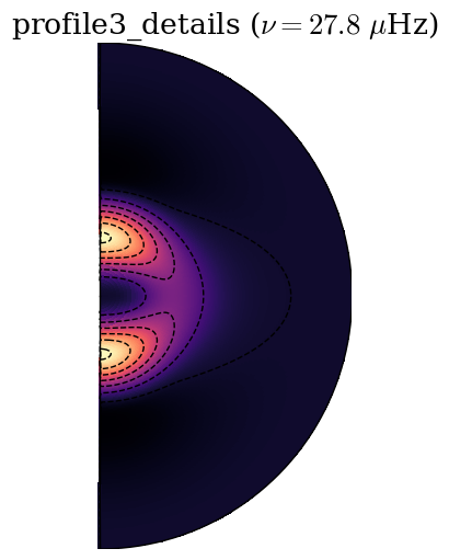
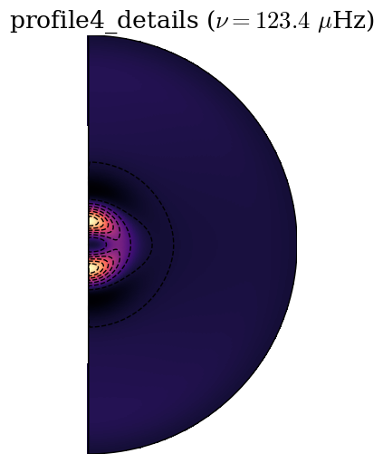
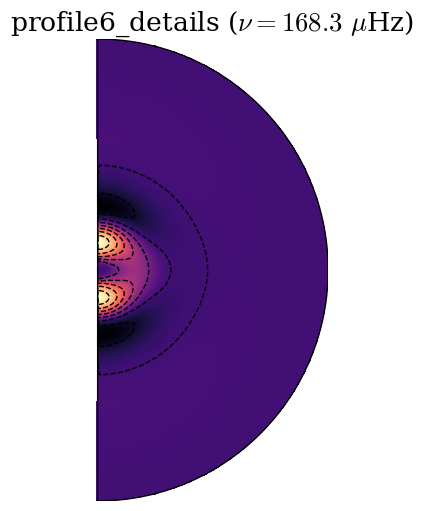
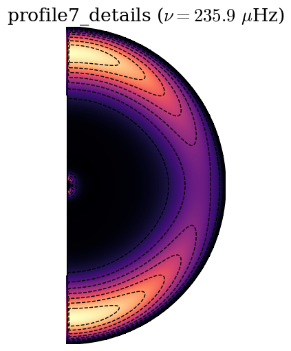
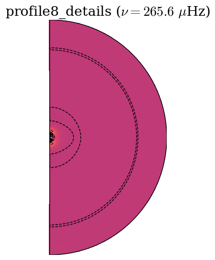
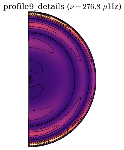
Finally, we can compute two-dimensional rotational kernels as a function of radius and latitude.

for details_dir in list_details :
    filename, file_exists = pph.grids.get_detail_file (details_dir, n=-1, l=1, m=1)
    if file_exists :
        d = pygyre.read_output(filename)
        (r, theta,
         beta_nlm, K_nlm) = pph_rot.compute_general_kernel (d["x"], d["rho"],
                                                            d["xi_r"], d["xi_h"],
                                                            l=d.meta["l"],
                                                            m=d.meta["m"],
                                                            theta_res=180, theta_1=180,
                                                            )
        title = r"{} ($\nu={:.1f}$ $\mu$Hz)".format (os.path.basename (details_dir),
                                                      d.meta["freq"].real)
        fig = pph_rot.plot_2D_kernel (r, theta, K_nlm, cmap="magma",
                                      title=title,
                                      #figsize=(4,4),
                                     )